Probabilistic Reasoning in Neural Networks: A Dev Guide

Introduction

Imagine deploying a medical image classifier that returns "Malignant: 87%" — but never tells you whether it’s 87% confident or just bluffing. Standard neural networks are notorious for this: they produce point estimates with no sense of their own doubt. A model trained on thousands of chest X-rays will happily output a confident prediction on a corrupted image, a rare disease variant, or data it has never seen before. That overconfidence is dangerous.

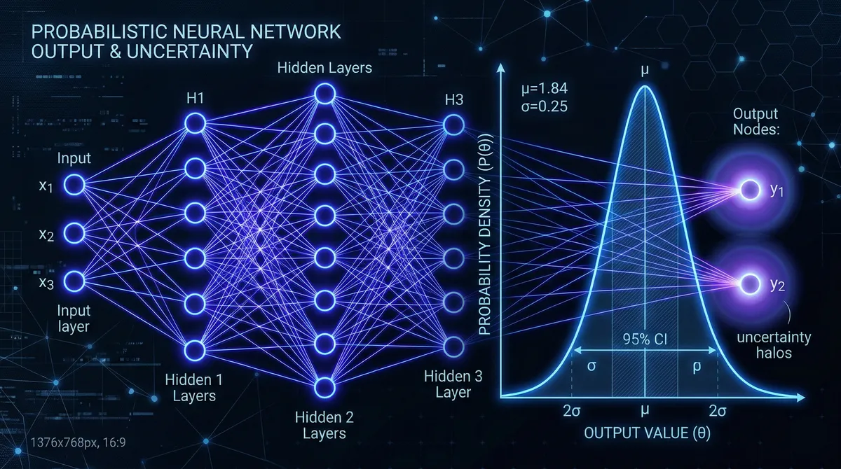
Probabilistic reasoning flips this around. Instead of asking “what is the answer?”, a probabilistic neural network asks “what is the distribution of possible answers, and how certain am I?” This is not just an academic nicety — it is how reliable AI systems are built for medicine, autonomous vehicles, robotics, and scientific discovery where being wrong (or overconfident) has real consequences.

In this guide you will learn the fundamental theory behind probabilistic neural networks, understand the two core types of uncertainty you need to care about, and build working implementations in PyTorch using three practical techniques: Bayesian Neural Networks (BNNs), MC Dropout, and Deep Ensembles. By the end you will be able to take an existing model and make it uncertainty-aware.

Prerequisites

• Comfortable with Python and PyTorch (tensors, autograd, nn.Module)
• Basic understanding of probability: distributions, Bayes’ theorem, expectations
• Familiarity with training a standard neural network
• Python 3.10+, PyTorch 2.3+, NumPy, Matplotlib

---

Core Concepts

What Is Probabilistic Reasoning?

A standard (deterministic) neural network learns a mapping f(x; θ) where θ are fixed weights. Given an input, it gives you one number. A probabilistic neural network instead learns a mapping over distributions: it reasons about p(y | x) — the full probability distribution over outputs given the input.

This is grounded in probability theory. The key ideas are:

Bayes’ theorem: p(θ | D) ∝ p(D | θ) · p(θ) — we update our belief about model parameters θ given observed data D, starting from a prior p(θ).

Predictive distribution: When making a prediction, we marginalize over all possible parameter settings: p(y | x, D) = ∫ p(y | x, θ) · p(θ | D) dθ. This integral is intractable for deep networks (millions of parameters), which is why we rely on approximations.

Aleatoric vs. Epistemic Uncertainty

This distinction is critical and often confused:

Mermaid diagram

Aleatoric uncertainty is irreducible — it is baked into the data generating process. If two doctors label the same ambiguous scan differently, no amount of additional data resolves that ambiguity.

Epistemic uncertainty is reducible — it reflects what the model doesn’t know because it hasn’t seen enough data. If you test a self-driving car in a snowstorm after training only on sunny roads, the model should express high epistemic uncertainty. Give it more snowy training data, and uncertainty drops.

Understanding which type of uncertainty dominates in a prediction is key to acting on it appropriately.

---

Method 1: MC Dropout (The Pragmatist’s BNN)

MC Dropout is the most practical entry point. The insight (from Gal & Ghahramani, 2016) is that a neural network with dropout applied at inference time — not just training — approximates Bayesian inference in a deep Gaussian process.

How it works: Run the same input through the network T times, each time with different neurons randomly dropped. The variance across these T stochastic forward passes estimates the model’s uncertainty.

import torch
import torch.nn as nn
import numpy as np

class MCDropoutRegressor(nn.Module):
    """
    Simple regressor with dropout that stays enabled at inference time.
    PyTorch 2.3+ compatible.
    """
    def __init__(self, input_dim: int, hidden_dim: int = 128, dropout_p: float = 0.1):
        super().__init__()
        self.net = nn.Sequential(
            nn.Linear(input_dim, hidden_dim),
            nn.ReLU(),
            nn.Dropout(p=dropout_p),   # <-- keep this active at test time
            nn.Linear(hidden_dim, hidden_dim),
            nn.ReLU(),
            nn.Dropout(p=dropout_p),
            nn.Linear(hidden_dim, 1),
        )

    def forward(self, x: torch.Tensor) -> torch.Tensor:
        return self.net(x)


def predict_with_uncertainty(
    model: nn.Module,
    x: torch.Tensor,
    n_samples: int = 100,
) -> tuple[torch.Tensor, torch.Tensor]:
    """
    MC Dropout inference: keep model in train() mode so Dropout fires.
    Returns (mean_prediction, std_prediction).
    """
    model.train()  # IMPORTANT: keeps Dropout active
    with torch.no_grad():
        preds = torch.stack([model(x) for _ in range(n_samples)], dim=0)  # [T, B, 1]

    mean = preds.mean(dim=0)   # [B, 1]
    std  = preds.std(dim=0)    # [B, 1] -- epistemic uncertainty estimate
    return mean, std


# --- Quick demo ---
torch.manual_seed(42)
model = MCDropoutRegressor(input_dim=1, dropout_p=0.05)
x_test = torch.linspace(-3, 3, 100).unsqueeze(1)

mean, std = predict_with_uncertainty(model, x_test, n_samples=200)
print(f"Mean range: [{mean.min():.3f}, {mean.max():.3f}]")
print(f"Std  range: [{std.min():.4f}, {std.max():.4f}]")
# Out-of-distribution points (far from training data) will show higher std

MC Dropout is fast to implement and adds almost no overhead to an existing architecture. The trade-off is that the uncertainty estimates can be poorly calibrated if dropout rate is poorly chosen. Start with p=0.05–0.1 for regression tasks.

---

Method 2: Bayesian Neural Networks with Variational Inference

A proper BNN replaces each weight w with a distribution q(w | μ, ρ) — typically a Gaussian parameterized by a mean μ and a log-variance ρ. During forward passes, weights are sampled from these distributions. Training maximizes the Evidence Lower BOund (ELBO), which balances likelihood of the data against a KL divergence term that regularizes the weight distributions toward the prior.

Intel Labs’ bayesian-torch library (v0.5+) makes this nearly plug-and-play:

pip install bayesian-torch torch torchvision

import torch
import torch.nn as nn
from bayesian_torch.models.dnn_to_bnn import dnn_to_bnn, get_kl_loss

# 1. Define a regular deterministic model
class DeterministicClassifier(nn.Module):
    def __init__(self, num_classes: int = 10):
        super().__init__()
        self.features = nn.Sequential(
            nn.Linear(784, 256),
            nn.ReLU(),
            nn.Linear(256, 128),
            nn.ReLU(),
        )
        self.classifier = nn.Linear(128, num_classes)

    def forward(self, x: torch.Tensor) -> torch.Tensor:
        return self.classifier(self.features(x.view(x.size(0), -1)))


# 2. Convert to Bayesian with a single API call
const_bnn_prior_parameters = {
    "prior_mu": 0.0,
    "prior_sigma": 1.0,
    "posterior_mu_init": 0.0,
    "posterior_rho_init": -3.0,
    "type": "Reparameterization",  # or "Flipout"
    "moped_enable": False,
}

det_model = DeterministicClassifier(num_classes=10)
dnn_to_bnn(det_model, const_bnn_prior_parameters)
# det_model is now a BNN -- all Linear layers replaced with BayesianLinear


# 3. Training loop with ELBO loss
optimizer = torch.optim.Adam(det_model.parameters(), lr=1e-3)
ce_loss = nn.CrossEntropyLoss()

def train_step(model, x_batch, y_batch, dataset_size: int):
    """
    ELBO = E[log p(y|x, w)] - KL[q(w) || p(w)]
    We estimate the KL term via get_kl_loss() and scale by dataset size.
    """
    model.train()
    optimizer.zero_grad()

    logits = model(x_batch)
    nll    = ce_loss(logits, y_batch)
    kl     = get_kl_loss(model) / dataset_size  # normalize by N

    elbo_loss = nll + kl
    elbo_loss.backward()
    optimizer.step()
    return elbo_loss.item(), nll.item()


# 4. Probabilistic inference (sample T weight draws)
def bnn_predict(model: nn.Module, x: torch.Tensor, n_samples: int = 50):
    model.eval()
    preds = []
    with torch.no_grad():
        for _ in range(n_samples):
            logits = model(x)
            probs  = torch.softmax(logits, dim=-1)
            preds.append(probs)

    preds = torch.stack(preds, dim=0)           # [T, B, C]
    mean_probs = preds.mean(dim=0)              # [B, C]

    # Predictive entropy = total uncertainty
    predictive_entropy = -(mean_probs * mean_probs.log()).sum(-1)

    # Mutual information = epistemic uncertainty
    entropy_of_mean = predictive_entropy
    mean_entropy    = -(preds * preds.log()).sum(-1).mean(0)
    mutual_info     = entropy_of_mean - mean_entropy

    return mean_probs, predictive_entropy, mutual_info

The KL term in the ELBO acts as a regularizer — it pulls weight distributions toward the prior, preventing overfitting and bounding model complexity.

---

Method 3: Deep Ensembles (Simple and Powerful)

Deep ensembles train M independent models with different random seeds and aggregate their predictions. Despite being “just” multiple networks, ensembles achieve excellent uncertainty calibration and are often competitive with (or better than) BNNs, as shown by Lakshminarayanan et al. (2017) and confirmed by benchmarks as recently as 2025.

import torch
import torch.nn as nn
from typing import List

class SimpleRegressor(nn.Module):
    def __init__(self, input_dim: int):
        super().__init__()
        # Two-head output: mean + log-variance (heteroscedastic regression)
        self.shared = nn.Sequential(
            nn.Linear(input_dim, 64), nn.ReLU(),
            nn.Linear(64, 64),        nn.ReLU(),
        )
        self.mean_head    = nn.Linear(64, 1)
        self.logvar_head  = nn.Linear(64, 1)

    def forward(self, x):
        h      = self.shared(x)
        mean   = self.mean_head(h)
        logvar = self.logvar_head(h)  # log σ² (aleatoric uncertainty)
        return mean, logvar


def gaussian_nll_loss(mean, logvar, target):
    """Negative log-likelihood for heteroscedastic Gaussian."""
    precision = torch.exp(-logvar)
    return 0.5 * (precision * (target - mean) ** 2 + logvar).mean()


class DeepEnsemble:
    """
    M independently trained models. Ensemble mean/variance capture
    both aleatoric (from each model's logvar head) and epistemic
    (from disagreement between models) uncertainty.
    """
    def __init__(self, models: List[nn.Module]):
        self.models = models

    @torch.no_grad()
    def predict(self, x: torch.Tensor):
        means, vars_ = [], []
        for m in self.models:
            m.eval()
            mu, logvar = m(x)
            means.append(mu)
            vars_.append(torch.exp(logvar))  # aleatoric variance per model

        means  = torch.stack(means)   # [M, B, 1]
        vars_  = torch.stack(vars_)   # [M, B, 1]

        ensemble_mean = means.mean(0)
        # Total variance = mean of variances + variance of means
        total_var = vars_.mean(0) + ((means - ensemble_mean) ** 2).mean(0)

        return ensemble_mean, total_var.sqrt()  # (mean, total std)


# Train M=5 models independently
M = 5
ensemble_models = [SimpleRegressor(input_dim=1) for _ in range(M)]
optimizers      = [torch.optim.Adam(m.parameters(), lr=1e-3) for m in ensemble_models]

# (training loop omitted for brevity — train each model on same dataset)

ensemble = DeepEnsemble(ensemble_models)
x_test   = torch.linspace(-3, 3, 100).unsqueeze(1)
pred_mean, pred_std = ensemble.predict(x_test)
print(f"Ensemble prediction: {pred_mean.squeeze()[:5]}")
print(f"Uncertainty (std):   {pred_std.squeeze()[:5]}")

The formula for total ensemble variance Var[y] = 𝔼[Var[y|θ]] + Var[𝔼[y|θ]] is a direct application of the law of total variance — aleatoric variance averaged across models, plus epistemic variance from model disagreement.

---

Practical Implementation: Medical Diagnosis Use Case

Here is how these ideas combine into a production-ready decision support pattern:

def make_clinical_decision(
    model,                    # BNN or ensemble
    image_tensor: torch.Tensor,
    uncertainty_threshold: float = 0.15,
    n_samples: int = 100,
) -> dict:
    """
    Returns a structured prediction with confidence and routing logic.
    High-uncertainty cases are flagged for expert review.
    """
    mean_probs, entropy, mutual_info = bnn_predict(model, image_tensor, n_samples)

    predicted_class  = mean_probs.argmax(dim=-1).item()
    confidence       = mean_probs.max(dim=-1).values.item()
    epistemic_unc    = mutual_info.item()

    needs_expert = epistemic_unc > uncertainty_threshold or confidence < 0.80

    return {
        "predicted_class":  predicted_class,
        "confidence":       round(confidence, 4),
        "epistemic_uncertainty": round(epistemic_unc, 4),
        "route_to_expert":  needs_expert,
        "reason": "High model uncertainty" if needs_expert else "Automated decision",
    }

This pattern — predict, quantify, route — is the core of responsible AI in high-stakes domains.

---

Calibration: Are Your Uncertainty Estimates Trustworthy?

A model is calibrated if, among all predictions where it says “80% confident,” about 80% are actually correct. Most standard neural networks are overconfident. You can diagnose this with a reliability diagram:

import numpy as np
import matplotlib.pyplot as plt

def reliability_diagram(confidences: np.ndarray, correctness: np.ndarray, n_bins: int = 10):
    """
    confidences: max softmax probability for each prediction [N]
    correctness: 1 if prediction was correct, 0 otherwise [N]
    """
    bins = np.linspace(0, 1, n_bins + 1)
    bin_acc, bin_conf = [], []

    for i in range(n_bins):
        mask = (confidences >= bins[i]) & (confidences < bins[i + 1])
        if mask.sum() > 0:
            bin_acc.append(correctness[mask].mean())
            bin_conf.append(confidences[mask].mean())

    bin_acc  = np.array(bin_acc)
    bin_conf = np.array(bin_conf)

    # Expected Calibration Error (ECE)
    ece = np.abs(bin_acc - bin_conf).mean()

    plt.figure(figsize=(6, 6))
    plt.plot([0, 1], [0, 1], "k--", label="Perfect calibration")
    plt.bar(bin_conf, bin_acc, width=0.08, alpha=0.7, label=f"Model (ECE={ece:.3f})")
    plt.xlabel("Confidence")
    plt.ylabel("Accuracy")
    plt.title("Reliability Diagram")
    plt.legend()
    plt.tight_layout()
    return ece

If your ECE is above 0.05 on a validation set, consider post-hoc calibration via temperature scaling — a single scalar T divides the logits before softmax to soften or sharpen the output distribution.

---

Common Pitfalls and Troubleshooting

BNN training doesn’t converge. This is the most common problem. The KL divergence term can dominate early in training, causing the posterior to collapse to the prior. Fix it by annealing the KL weight from 0 → 1 over the first few epochs (KL annealing / β-VAE schedule).

MC Dropout gives near-zero variance. Your dropout probability is too low, or the model is underfitting. Try raising dropout_p to 0.1–0.2 and ensure you call model.train() (not model.eval()) at inference time.

Ensemble members give identical predictions. They weren’t initialized differently enough, or training data was too deterministic. Ensure each model uses a different random seed and shuffled data ordering.

Uncertainty doesn’t increase on out-of-distribution data. This is a known failure mode of softmax-based models. The softmax function can produce confident-looking outputs even for completely novel inputs. Use energy-based OOD detection or distance-aware methods (Deep Deterministic Uncertainty, DUQ) for more robust OOD detection.

Slow inference with large ensembles. Consider “Packed Ensembles” (Laurent et al., ICLR 2023), which pack multiple sub-networks into a single forward pass using grouped convolutions, cutting compute by 3–5×.

---

Choosing the Right Method

Method	Calibration	Cost	Best For
MC Dropout	Moderate	Low	Quick retrofit on existing model
BNN (VI)	Good	Medium	When interpretable priors matter
Deep Ensembles	Best	High (×M compute)	Production, safety-critical
Temperature Scaling	Good (post-hoc)	Minimal	Calibrating any existing model

---

Conclusion

Probabilistic reasoning transforms neural networks from opaque point-estimators into transparent, calibrated reasoners that know what they don’t know. The core ideas are straightforward: treat weights (or outputs) as distributions, sample to approximate intractable integrals, and decompose uncertainty into its aleatoric and epistemic components.

For most teams, the practical journey looks like: (1) add MC Dropout to your existing model as a baseline, (2) evaluate calibration with ECE and reliability diagrams, (3) graduate to deep ensembles or BNNs when the application demands tighter uncertainty control. The bayesian-torch and torch-uncertainty libraries make steps 2 and 3 far more accessible than they were even two years ago.

The payoff extends beyond safety: uncertainty-aware models enable active learning (label the most uncertain points), adaptive inference (skip expensive computation when the model is already confident), and better human-AI teaming (route uncertain cases to experts).

---

References:

1. Intel Labs – Bayesian-Torch Library — https://github.com/IntelLabs/bayesian-torch — Library documentation and usage for BNN layers in PyTorch
2. Torch-Uncertainty (NeurIPS 2025, Spotlight) — https://openreview.net/forum?id=oYfRRQr9uK — Unified PyTorch framework benchmarking UQ methods across tasks
3. AI4Fusion Summer School 2025 – Basic BNN with PyTorch — https://ai4fusion-wmschool.github.io/summer2025/Lecture17_BasicBNN.html — Practical MC Dropout tutorial with classification examples
4. Bayesian Network Modeling for Probabilistic Reasoning (IJSRA, 2025) — https://journalijsra.com/sites/default/files/fulltext_pdf/IJSRA-2025-1765.pdf — Survey of BN-based reasoning for industrial datasets, aleatoric vs. epistemic framing
5. EmergentMind – Probabilistic Deep Learning Models — https://www.emergentmind.com/topics/probabilistic-deep-learning-models — Overview of DPMs, VAEs, variational inference, and probabilistic programming